Friday, January 6, 2012

El Niño, La Niña and the Southern Oscillation

El Niño is the name given to the occasional development of warm ocean surface waters along the coast of Ecuador and Peru. When this warming occurs the usual upwelling of cold, nutrient rich deep ocean water is significantly reduced. El Niño normally occurs around Christmas and usually lasts for a few weeks to a few months. Sometimes an extremely warm event can develop that lasts for much longer time periods. In the 1990s, strong El Niños developed in 1991 and lasted until 1995, and from fall 1997 to spring 1998.

The formation of an El Niño is linked with the cycling of a Pacific Ocean circulation pattern known as the southern oscillation. In a normal year, a surface low pressure develops in the region of northern Australia and Indonesia and a high pressure system over the coast of Peru (see Figure 7z-1 below). As a result, the trade winds over the Pacific Ocean move strongly from east to west. The easterly flow of the trade winds carries warm surface waters westward, bringing convective storms to Indonesia and coastal Australia. Along the coast of Peru, cold bottom water wells up to the surface to replace the warm water that is pulled to the west.


Figure 7z-1: This cross-section of the Pacific Ocean, along the equator, illustrates the pattern of atmospheric circulation typically found at the equatorial Pacific. Note the position of the thermocline.

In an El Niño year, air pressure drops over large areas of the central Pacific and along the coast of South America (see Figure 7z-2 below). The normal low pressure system is replaced by a weak high in the western Pacific (the southern oscillation). This change in pressure pattern causes the trade winds to be reduced. This reduction allows the equatorial counter current (which flows west to east) to accumulate warm ocean water along the coastlines of Peru and Ecuador (Figure 7z-3). This accumulation of warm water causes the thermocline to drop in the eastern part of Pacific Ocean which cuts off the upwelling of cold deep ocean water along the coast of Peru. Climatically, the development of an El Niño brings drought to the western Pacific, rains to the equatorial coast of South America, and convective storms and hurricanes to the central Pacific.


Figure 7z-2: This cross-section of the Pacific Ocean, along the equator, illustrates the pattern of atmospheric circulation that causes the formation of the El Niño. Note how position of the thermocline has changed from Figure 7z-1.


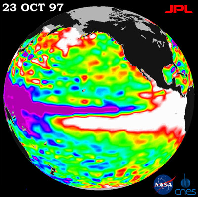
Figure 7z-3: NASA's TOPEX/Poseidon satellite is being used to monitor the presence of El Niño. Sensors on the satellite measure the height of the Pacific Ocean. The scale below describes the relationship between image color and the relative surface height of the ocean. In the image above, we can see the presence of a strong El Niño event in the eastern Pacific (October, 1997). The presence of the El Niño causes the height of the ocean along the equator to increase from the middle of the image to the coastline of Central and South America. (Source: NASA - TOPEX/Poseidon).

CAUSES OF CLIMATE CHANGE

Figure 7y-1 illustrates the basic components that influence the state of the Earth's climatic system. Changes in the state of this system can occur externally (from extraterrestrial systems) or internally (from ocean, atmosphere and land systems) through any one of the described components. For example, an external change may involve a variation in the Sun's output which would externally vary the amount of solar radiation received by the Earth's atmosphere and surface. Internal variations in the Earth's climatic system may be caused by changes in the concentrations of atmospheric gases, mountain building, volcanic activity, and changes in surface or atmospheric albedo.


Figure 7y-1: Factors that influence the Earth's climate.

The work of climatologists has found evidence to suggest that only a limited number of factors are primarily responsible for most of the past episodes of climate change on the Earth. These factors include:

  • Variations in the Earth's orbital characteristics.
  • Atmospheric carbon dioxide variations.
  • Volcanic eruptions
  • Variations in solar output.
Variations in the Earth's Orbital Characteristics
The Milankovitch theory suggests that normal cyclical variations in three of the Earth's orbital characteristics is probably responsible for some past climatic change. The basic idea behind this theory assumes that over time these three cyclic events vary the amount of solar radiation that is received on the Earth's surface.

The first cyclical variation, known as eccentricity, controls the shape of the Earth's orbit around the Sun. The orbit gradually changes from being elliptical to being nearly circular and then back to elliptical in a period of about 100,000 years. The greater the eccentricity of the orbit (i.e., the more elliptical it is), the greater the variation in solar energy received at the top of the atmosphere between the Earth's closest (perihelion) and farthest (aphelion) approach to the Sun. 

EARTH'S CLIMATIC HISTORY

Reconstructing Past Climates
A wide range of evidence exists to allow climatologists to reconstruct the Earth's past climate. This evidence can be grouped into three general categories.

The first category is meteorological instrument records. Common climatic elements measured by instruments include temperature, precipitation, wind speed, wind direction, and atmospheric pressure. However, many of these records are temporally quite short as many of the instruments used were only created and put into operation during the last few centuries or decades. Another problem with instrumental records is that large areas of the Earth are not monitored. 

Most of the instrumental records are for locations in populated areas of Europe and North America. Very few records exist for locations in less developed countries (LDCs), in areas with low human populations, and the Earth's oceans. Over the last half century many meteorological stations have been added in land areas previously not covered. Another important advancement in developing a global record of climate has been the recent use of remote satellites.

Written documentation and descriptive accounts of the weather make up the second general category of evidence for determining climate change. Weather phenomena commonly described in this type of data includes the prevailing character of the seasons of individual years, reports of floods, droughts, great frosts, periods of bitter cold, and heavy snowfalls. Large problems exist in the interpretation of this data because of its subjective nature.

INTRODUCTION TO APPLIED CLIMATOLOGY


Urban Climatology
Urban and rural environments differ substantially in their micro-climate. These climatic differences are primarily caused by the alteration of the Earth's surface by human construction and the release of artificially created energy into the environment.

Energy Characteristics of Urban Areas
In a city, concrete, asphalt, and glass replace natural vegetation, and vertical surfaces of buildings are added to the normally flat natural rural landscape. Urban surfaces generally have a lower albedo, greater heat conduction, and more heat storage than the surfaces they replaced. The geometry of city buildings causes the absorption of a greater quantity of available incoming solar radiation and outgoing terrestrial infrared radiation. Even in early morning and late afternoon the urban areas are intercepting and absorbing radiation on their vertical surfaces. 

In urban areas, large amounts of heat energy are added to the local energy balance through transportation, industrial activity, and the heating of buildings. In winter, the amount of heat generated from the burning of fossil fuels in New York City is 2.5 times greater than the heat absorbed from the Sun. Finally, in rural areas, evaporation and transpiration from various natural surfaces act to cool the land surface and local atmosphere. In urban locations, drainage systems have been created to quickly remove surface water. Thus, little water is available for cooling.

CLIMATE CLASSIFICATION AND CLIMATIC REGIONS OF THE WORLD

Climate Classification

The Köppen Climate Classification System is the most widely used system for classifying the world's climates. Its categories are based on the annual and monthly averages of temperature and precipitation. The Köppen system recognizes five major climatic types; each type is designated by a capital letter.


A - Tropical Moist Climates: all months have average temperatures above 18° Celsius.


B - Dry Climates: with deficient precipitation during most of the year.

C - Moist Mid-latitude Climates with Mild Winters.

D - Moist Mid-Latitude Climates with Cold Winters.

E - Polar Climates: with extremely cold winters and summers.


Tropical Moist Climates (A)
Tropical moist climates extend northward and southward from the equator to about 15 to 25° of latitude. In these climates all months have average temperatures greater than 18° Celsius. Annual precipitation is greater than 1500 mm. Three minor Köppen climate types exist in the A group, and their designation is based on seasonal distribution of rainfall. Af or tropical wet is a tropical climate where precipitation occurs all year long. Monthly temperature variations in this climate are less than 3° Celsius. Because of intense surface heating and high humidity, cumulus and cumulonimbus clouds form early in the afternoons almost every day. Daily highs are about 32° Celsius, while night time temperatures average 22° Celsius. Am is a tropical monsoon climate. Annual rainfall is equal to or greater than Af, but most of the precipitation falls in the 7 to 9 hottest months. During the dry season very little rainfall occurs. The tropical wet and dry or savanna (Aw) has an extended dry season during winter. Precipitation during the wet season is usually less than 1000 millimeters, and only during the summer season.

TROPICAL WEATHER AND HURRICANES

Tropical Weather
The tropics can be defined as the area of the Earth found between the Tropic of Cancer (23.5° North) and the Tropic Capricorn (23.5° South). In this region, the Sun will be directly overhead during some part of the year. The temperature of the tropics does not vary much from season to season because high quantities of solar insolation are received here regardless of the time of the year. Weather in the tropics is dominated by convective storms that develop mainly along the intertropical convergence zone (ITCZ), the subtropical high pressure zone, and oceanic disturbances in the trade winds that sometimes develop into hurricanes.

One of the most important weather features found in the tropics is the intertropical convergence zone. The intertropical convergence zone is distinguished by a wide band of cumulus and cumulonimbus clouds that are created by dynamic atmospheric lifting due to convergence and convection. In general, the intertropical convergence zone delineates the location where the noonday Sun is directly overhead. Because of the high Sun, the intertropical convergence zone receives the greatest quantity of daily solar insolation in the tropics. 

At the intertropical convergence zone, this energy is used to evaporate large amounts of water and is converted into sensible heat at the ground surface and within the atmosphere. Often, these processes lead to an almost daily development of convective thunderstorms by providing moisture and heat for the development of cumulonimbus clouds. The intertropical convergence zone also represents the location of convergence of the northeast and southeast trade winds. The convergence of these wind systems enhances the development of convective rain clouds at the tropics.

The intertropical convergence zone moves seasonally with the tilt of the Earth's axis. The convective rains that accompany the passage of the intertropical convergence zone are the primary source of precipitation for locations roughly 10 to 23.5° North and South latitude. Figure 7u-1describes the seasonal movement of the intertropical convergence zone and other systems associated with our planet’s global circulation.


Figure 7u-1: Seasonal movement of the Earth's global circulation patterns. The major circulation cells are identified on the “Equinox” figure. In the “Equinox” figure, the intertropical convergence zone (ITCZ) occurs at the equator where the Trade Winds converge creating a low-pressure center and updrafts (red arrows). The upward movement of the moist tropical air above the intertropical convergence zone produces a band of thunderstorm activity that brings precipitation to the tropics. At the zone where the Hadley Cell and Ferrel Cell meet, tropospheric airflow is in a downward direction moving from the top of the troposphere to the Earth’s surface (green arrows). These downdrafts give rise to the subtropical high-pressure zone on the Earth’s surface. Surface air also moves upward into the troposphere at the boundary between the Ferrel Cell and the Polar Cell. At this location, frontal lifting associated with mid-latitude cyclones moves warm subtropical air over cold polar air producing clouds and precipitation. Note how the Earth’s circulation patterns change their position in the December and June solstice figures.

THUNDERSTORMS AND TORNADOES

 Thunderstorms
Thunderstorms form when moist, unstable air is lifted vertically into the atmosphere. Lifting of this air results in condensation and the release of latent heat. The process to initiate vertical lifting can be caused by:

(1). Unequal warming of the surface of the Earth.

(2). Orographic lifting due to topographic obstruction of air flow.

(3). Dynamic lifting because of the presence of a frontal zone.

Immediately after lifting begins, the rising parcel of warm moist air begins to cool because of adiabatic expansion. At a certain elevation the dew point is reached resulting in condensation and the formation of a cumulus cloud. For the cumulus cloud to form into a thunderstorm, continued uplift must occur in an unstable atmosphere. With the vertical extension of the air parcel, the cumulus cloud grows into a cumulonimbus cloud. Cumulonimbus clouds can reach heights of 20 kilometers above the Earth's surface. Severe weather associated with some these clouds includes hail, strong winds, thunder, lightning, intense rain, and tornadoes.


Figure 7t-1: Hail stone measuring 6 centimeters in diameter. (Source: NOAA Photo Library - National Severe Storms Laboratory).


Figure 7t-2: Multiple lightning strikes from a thunderstorm occurring at night. (Source: NOAA Photo Library - National Severe Storms Laboratory).


Generally, two types of thunderstorms are common:

1) Air mass thunderstorms which occur in the mid-latitudes in summer and at the equator all year long.

2) Thunderstorms associated with mid-latitude cyclone cold fronts or dry lines. This type of thunderstorm often has severe weather associated with it.

The most common type of thunderstorm is the air mass storm. Air mass thunderstorms normally develop in late afternoon hours when surface heating produces the maximum number of convection currents in the atmosphere. The life cycle of these weather events has three distinct stages. The first stage of air mass thunderstorm development is called the cumulus stage (Figure 7t-3). In this stage, parcels of warm humid air rise and cool to form clusters of puffy white cumulus clouds. The clouds are the result of condensation and deposition which releases large quantities of latent heat. The added heat energy keeps the air inside the cloud warmer than the air around it. The cloud continues to develop as long as more humid air is added to it from below. Updrafts dominate the circulation patterns within the cloud.


Figure 7t-3: Developing thunderstorm cloud at the cumulus stage.


When the updrafts reach their maximum altitude in the developing cloud, usually 12 to 14 kilometers, they change their direction 180° and become downdrafts. This marks the mature stage (Figure 7t-4). With the downdrafts, precipitation begins to form through collision and coalescence (Figure 7t-5). The storm is also at its most intense stage of development and is now a cumulonimbus cloud The top of the cloud takes on the familiar anvil shape, as strong stratospheric upper-level winds spread ice crystals in the top of the cloud horizontally. At its base, the thunderstorm is several kilometers in diameter. The mature air mass thunderstorm contains heavy rain, thunder, lightning, and produces wind gusts at the surface.


Figure 7t-4: Mature thunderstorm cloud with typical anvil shaped cloud.


Figure 7t-5: Downdrafts from this mature thunderstorm are moving air and rain from the cloud to the ground surface (Photo © 2004 David Jenkins).

The mature thunderstorm begins to decrease in intensity and enters the dissipating stage after about half an hour. Air currents within the convective storm are now mainly downdrafts as the supply of warm moist air from the lower atmosphere is depleted. Within about 1 hour, the storm is finished and precipitation has stopped.

THE MID - LATITUDE CYCLONE

Mid-latitude or frontal cyclones are large traveling atmospheric cyclonic storms up to 2000 kilometers in diameter with centers of low atmospheric pressure. An intense mid-latitude cyclone may have a surface pressure as low as 970 millibars, compared to an average sea-level pressure of 1013 millibars. Normally, individual frontal cyclones exist for about 3 to 10 days moving in a generally west to east direction. Frontal cyclones are the dominant weather event of the Earth's mid-latitudes forming along the polar front. (Figure 7s-1).


Figure 7s-1: A series of mid-latitude cyclones forming along the polar front (black line with red half circle and blue triangle symbols). On the illustration, the low pressure center of the mid-latitude cyclones is identfied by a red L. The systems located along the west and east coast of North America are in the middle stage of their life. The mid-latitude cyclone east of Greenland is at the end of its life cycle. In their mature stage, mid-latitude cyclones have a warm front on the east side of the storm's center and a cold front to the west. The cold front travels faster than the warm front. Near the end of the storm's life the cold front catches up to the warm front causing a condition known as occlusion.


Mid-latitude cyclones are the result of the dynamic interaction of warm tropical and cold polar air masses at the polar front. This interaction causes the warm air to be cyclonically lifted vertically into the atmosphere where it combines with colder upper atmosphere air. This process also helps to transport excess energy from the lower latitudes to the higher latitudes.

The mid-latitude cyclone is rarely motionless and commonly travels about 1200 kilometers in one day. Its direction of movement is generally eastward (Figure 7s-2). Precise movement of this weather system is controlled by the orientation of the polar jet stream in the upper troposphere. An estimate of future movement of the mid-latitude cyclone can be determined by the winds directly behind the cold front. If the winds are 70 kilometers per hour, the cyclone can be projected to continue its movement along the ground surface at this velocity.

Figure 7s-2: Typical paths of mid-latitude cyclones are represented by black arrows. This image also shows the typical paths traveled by subtropical hurricanes (green arrows).

Figure 7s-3 describes the patterns of wind flow, surface pressure, fronts, and zones of precipitation associated with a mid-latitude cyclone in the Northern Hemisphere. Around the low, winds blow counterclockwise and inwards (clockwise and inward in the Southern Hemisphere). West of the low, cold air traveling from the north and northwest creates a cold front extending from the cyclone's center to the southwest. Southeast of the low, northward moving warm air from the subtropics produces a warm front. Precipitation is located at the center of the low and along the fronts where air is being uplifted.

Mid-latitude cyclones can produce a wide variety of precipitation types. Precipitation types include: rain, freezing rain, hail, sleet, snow pellets, and snow. Frozen forms of precipitation (except hail) are common with storms that occur in the winter months. Hail is associated with severe thunderstorms that form along or in front of cold fronts during spring and summer months.


Figure 7s-3: Fronts, winds patterns, pressure patterns, and precipitation distribution found in an idealized mature mid-latitude cyclone.

Figure 7s-4 describes a vertical cross-section through a mature mid-latitude cyclone. In this cross-section, we can see how air temperature changes as we move from behind the cold front to a position ahead of the warm front. Behind the surface position of the cold front, forward moving cold dense air causes the uplift of the warm lighter air in advance of the front. Because this uplift is relatively rapid along a steep frontal gradient, the condensed water vapor quickly organizes itself into cumulus and then cumulonimbus clouds. Cumulonimbus clouds produce heavy precipitation and can develop into severe thunderstorms if conditions are right. Along the gently sloping warm front, the lifting of moist air produces first nimbostratus clouds followed by altostratus and cirrostratus. Precipitation is less intense along this front, varying from moderate to light showers some distance ahead of the surface location of the warm front.


Figure 7s-4: Vertical cross-section of the line A-B in Figure 7s-3.


Frontal cyclone development is related to polar jet stream processes. Within the jet stream, localized areas of air outflow can occur because of upper air divergence. Outflow results in the development of an upper air vacuum. To compensate for the vacuum in the upper atmosphere, surface air flows cyclonically upward into the outflow to replenish lost mass. The process stops and the mid-latitude cyclone dissipates when the upper air vacuum is filled with surface air.

AIR MASSES AND FRONTAL TRANSITIONAL ZONE

An air mass is a large body of air of relatively similar temperature and humidity characteristics covering thousands of square kilometers. Typically, air masses are classified according to the characteristics of their source region or area of formation. A source region can have one of four temperature attributes: equatorial, tropical, polar or arctic. Air masses are also classified as being either continental or maritime in terms of moisture characteristics. Combining these two categories, several possibilities are commonly found associated with North America: maritime polar (mP), continental polar (cP), maritime tropical (mT), continental tropical (cT), and continental arctic (A). The following diagram(Figure 7r-1) describes the source regions and common patterns of movement for the various types of air masses associated with North America.


Figure 7r-1: Source sites and movement patterns for North America's major air masses.


Frequently, two air masses, especially in the middle latitudes, develop a sharp boundary or interface, where the temperature difference between them becomes intensified. Such an area of intensification is called a frontal zone or a front. The boundary between the warm and cold air masses always slopes upwards over the cold air. This is due to the fact that cold air is much denser than warm air. The sloping of warm air over the cold air leads to a forced uplifting (frontal lifting) of the warm air if one air mass is moving toward the other. In turn, this uplifting causes condensation to occur and the possibility of precipitation along the frontal boundary.

Frontal zones where the air masses are not moving against each other are called stationary fronts. In transitional areas where there is some air mass movement, cold or warm fronts can develop. Figure 7r-2 illustrates a vertical cross-section of a cold front. A cold front is the transition zone in the atmosphere where an advancing cold, dry stable air mass displaces a warm, moist unstable subtropical air mass. On a weather map, the cold front is drawn as a solid blue line with triangles. The position of the triangles shows the direction of frontal movement. Cold fronts move between 15 to 50 kilometers per hour in a southeast to east direction. The formation of clouds and precipitation at the frontal zone is caused by frontal lifting. High altitude cirrus clouds are found well in advance of the front. Above the surface location of the cold front, high altitude cirrostratus and middle altitude altocumulus are common. Precipitation is normally found just behind the front where frontal lifting has caused the development of towering cumulus and cumulonimbus clouds. Table 7r-1 describes some of the weather conditions associated with a cold front.

Table 7r-1: Weather conditions associated with a cold front.
Weather Phenomenon
Prior to the Passing of the Front
Contact with the Front
After the Passing of the Front
TemperatureWarmCooling suddenlyCold and getting colder
Atmospheric PressureDecreasing steadilyLeveling off then increasingIncreasing steadily
WindsSouth to southeastVariable and gustyWest to northwest
PrecipitationShowersHeavy rain or snow, hail sometimesShowers then clearing
CloudsCirrus and cirrostratus changing later to cumulus and cumulonimbusCumulus and cumulonimbusCumulus


Figure 7r-2: Atmospheric cross-section of a cold front.


A warm front is illustrated in the cross-section diagram below (Figure 7r-3). A warm front is the transition zone in the atmosphere where an advancing warm subtropical, moist air mass replaces a retreating cold, dry polar air mass. On a weather map, a warm front is drawn as a solid red line with half-circles. The position of the half-circles shows the direction of frontal movement. Warm fronts move about 10 kilometers per hour in a northeast direction. 

Thursday, January 5, 2012

UPPER AIR WINDS AND THE JET STREAM

Winds at the top of the troposphere are generally pole ward and westerly in direction. Figure 7q-1 describes these upper air westerlies along with some other associated weather features. Three zones of westerlies can be seen in each hemisphere on this illustration. Each zone is associated with either the Hadley, Ferrel, or Polar circulation cell.


Figure 7q-1: Simplified global three-cell upper air circulation patterns.


The polar jet stream is formed by the deflection of upper air winds by coriolis acceleration (see Figure 7q-3 below). It resembles a stream of water moving west to east and has an altitude of about 10 kilometers. Its air flow is intensified by the strong temperature and pressure gradient that develops when cold air from the poles meets warm air from the tropics. Wind velocity is highest in the core of the polar jet stream where speeds can be as high as 300 kilometers per hour. The jet stream core is surrounded by slower moving air that has an average velocity of 130 kilometers per hour in winter and 65 kilometers per hour in summer.

GLOBAL SCALE CIRCULATION OF THE ATMOSPHERE

Simple Model of Global Circulation

We can gain an understanding of how global circulation works by developing two simplified graphical models of processes that produce this system. The first model will be founded on the following simplifying assumptions:

  • The Earth is not rotating in space.
  • The Earth's surface is composed of similar materials.
  • The global reception of solar insolation and loss of longwave radiation cause a temperature gradient of hotter air at the equator and colder air at the poles.

Based on these assumptions, air circulation on the Earth should approximate the patterns shown on Figure 7p-1. In this illustration, each hemisphere contains one three-dimensional circulation cell.


Figure 7p-1: Simplified one-cell global air circulation patterns.


As described in the diagram above, surface air flow is from the poles to the equator. When the air reaches the equator, it is lifted vertically by the processes of convection and convergence. When it reaches the top of the troposphere, it begins to flow once again horizontally. However, the direction of flow is now from the equator to the poles. At the poles, the air in the upper atmosphere then descends to the Earth's surface to complete the cycle of flow.


LOCAL AND REGIONAL WIND SYSTEMS

Thermal Circulations
winds blow because of differences in atmospheric pressure. Pressure gradients may develop on a local to a global scale because of differences in the heating and cooling of the Earth's surface. Heating and cooling cycles that develop daily or annually can create several common local or regional thermal wind systems. The basic circulation system that develops is described in the generic illustrations below.


Figure 7o-1: Cross-section of the atmosphere with uniform horizontal atmospheric pressure.

In this first diagram (Figure 7o-1), there is no horizontal temperature or pressure gradient and therefore no wind. Atmospheric pressure decreases with altitude as depicted by the drawn isobars (1000 to 980 millibars). In the second diagram (Figure 7o-2), the potential for solar heating is added which creates contrasting surface areas of temperature and atmospheric pressure. The area to the right receives more solar radiation and the air begins to warm from heat energy transferred from the ground through conduction and convection. The vertical distance between the isobars becomes greater as the air rises. To the far left, less radiation is received because of the presence of cloud, and this area becomes relatively cooler than the area to the right. In the upper atmosphere, a pressure gradient begins to form because of the rising air and upward spreading of the isobars. The air then begins to flow in the upper atmosphere from high pressure to low pressure.


Figure 7o-2: Development of air flow in the upper atmosphere because of surface heating.

Figure 7o-3 shows the full circulation system in action. Beneath the upper atmosphere high is a thermal low pressure center created from the heating of the ground surface. Below the upper atmosphere low is a thermal high created by the relatively cooler air temperatures and enhanced by the descending air from above. Surface air temperatures are cooler here because of the obstruction of shortwave radiation absorption at the Earth's surface by the cloud. At the surface, the wind blows from the high to the low pressure. Once at the low, the wind rises up to the upper air high pressure system because of thermal buoyancy and outflow in the upper atmosphere. From the upper high, the air then travels to the upper air low, and then back down to the surface high to complete the circulation cell. The circulation cell is a closed system that redistributes air in an equitable manner. It is driven by the greater heating of the surface air in the right of the diagram.


Figure 7o-3: Development of a closed atmospheric circulation cell because of surface heating.


FORCES ACTING TO CREATE WIND

Wind can be defined simply as air in motion. This motion can be in any direction, but in most cases the horizontal component of wind flow greatly exceeds the flow that occurs vertically. The speed of wind varies from absolute calm to speeds as high as 380 kilometers per hour (Mt. Washington, New Hampshire, April 12, 1934). In 1894, strong winds in Nebraska pushed six fully loaded coal cars over 160 kilometers in just over three hours. Over short periods of time surface winds can be quite variable.


Wind develops as a result of spatial differences in atmospheric pressure. Generally, these differences occur because of uneven absorption of solar radiation at the Earth's surface (Figure 7n-1). Wind speed tends to be at its greatest during the daytime when the greatest spatial extremes in atmospheric temperature and pressure exist.


Figure 7n-1: Formation of wind as a result of localized temperature differences.


Wind is often described by two characteristics: wind speed and wind direction. Wind speed is the velocity attained by a mass of air traveling horizontally through the atmosphere. Wind speed is often measured with an anemometer in kilometers per hour (kmph), miles per hour (mph), knots, or meters per second (mps) (Figure 7n-2). Wind direction is measured as the direction from where a wind comes from. For example, a southerly wind comes from the south and blows to the north. Direction is measured by an instrument called a wind vane (Figure 7n-2). Both of these instruments are positioned in the atmospheric environment at a standard distance of 10 meters above the ground surface.

GLOBAL SURFACE TEMPERATURE DISTRIBUTION

If the Earth was a homogeneous body without the present land/ocean distribution, its temperature distribution would be strictly latitudinal (Figure 7m-1). However, the Earth is more complex than this being composed of a mosaic of land and water. This mosaic causes latitudinal zonation of temperature to be disrupted spatially.


Figure 7m-1: Simple latitudinal zonation of temperature.


The following two factors are important in influencing the distribution of temperature on the Earth's surface:


  • The latitude of the location determines how much solar radiation is received. Latitude influences the angle of incidence and duration of day length.
  • Surface properties - surfaces with high albedo absorb less incident radiation. In general, land absorbs less insolation that water because of its lighter color. Also, even if two surfaces have the same albedo, a surface's specific heat determines the amount of heat energy required for a specific rise in temperature per unit mass. The specific heat of water is some five times greater than that of rock and the land surface (see Table 7m-1 below). As a result, water requires the input of large amounts of energy to cause a rise in its temperature.

Table 7m-1: Specific Heat of Various Substances.

 Substance
Specific Heat
 Water
 1.00
 Air
 0.24
 Granite
 0.19
 Sand
 0.19
 Iron
 0.11


Mainly because of specific heat, land surfaces behave quite differently from water surfaces. In general, the surface of any extensive deep body of water heats more slowly and cools more slowly than the surface of a large land body. Other factors influencing the way land and water surfaces heat and cool include:

  • Solar radiation warms an extensive layer in water, on land just the immediate surface is heated.
  • Water is easily mixed by the process of convection.
  • Evaporation of water removes energy from water's surface.


DAILY AND ANNUAL CYCLES OF TEMPERATURE

Daily Cycles of Air Temperature

At the Earth's surface quantities of insolation and net radiation undergo daily cycles of change because the planet rotates on its polar axis once every 24 hours. Insolation is usually the main positive component making up net radiation. Variations in net radiation are primarily responsible for the particular patterns of rising and falling air temperature over a 24 hour period. The following three graphs show hypothetical average curves of insolation, net radiation, and air temperature for a typical land based location at 45° of latitude on the equinoxes and solstices(Figures 1, 2, and 3).


Insolation


Figure 1: Hourly variations in insolation received for a location at 45° North latitude over a 24 hour period.

In the above graph, shortwave radiation received from the Sun is measured in Watts. For all dates, peak reception occurs at solar noon when the Sun attains its greatest height above the horizon.


Net Radiation

Figure 2: Hourly variations in net radiation for a location at 45° North latitude over a 24 hour period.

Units in Figure 2 are the same as the insolation graph above. The net radiation graph indicates that there is a surplus of radiation during most of the day and a deficit throughout the night. The deficit begins just before sunset when emitted longwave radiation from the Earth's surface exceeds solar insolation and longwave radiation from the atmosphere.

Temperature


Figure 3: Hourly variations in surface temperature for a location at 45° North latitude over a 24 hour period.


THE CONCEPT OF TEMPERATURE

Temperature and Heat
Temperature and heat are not the same phenomenon. Temperature is a measure of the intensity or degree of hotness in a body. Technically, it is determined by getting the average speed of a body's molecules. Heat is a measure of the quantity of heat energy present in a body. The spatial distribution of temperature in a body determines heat flow. Heat always flows from warmer to colder areas.

The heat held in a object depends not only on its temperature but also its mass. For example, let us compare the heating of two different masses of water (Table 7k-1). In this example, one mass has a weight of 5 grams, while the other is 25 grams. If the temperature of both masses is raised from 20 to 25° Celsius, the larger mass of water will require five times more heat energy for this increase in temperature. This larger mass would also contain contain 5 times more stored heat energy.

Table 7k-1: Heat energy required to raise two different quantities of water 5° Celsius.
 Mass of the Water Starting Temperature Ending Temperature Heat Required
 5 grams 20° Celsius 25° Celsius 25 Calories of Heat
 25 grams 20° Celsius 25° Celsius 125 Calories of Heat

Temperature Scales
A number of measurement scales have been invented to measure temperature. Table 7k-2 describes important temperatures for the three dominant scales in use today.

Table 7k-2: Temperature of absolute zero, the ice point of water, and the stream point of water using various temperature measurement scales.
 Measurement Scale
 Steam Point of Water
 Ice Point of Water
 Absolute Zero
 Fahrenheit
 212
 32
 -460
 Celsius
 100
 0
 -273
 Kelvin
 373
 273
 0


The most commonly used scale for measuring temperature is the Celsius system. The Celsius scale was developed in 1742 by the Swedish astronomer Andres Celsius. In this system, the melting point of ice was given a value of 0, the boiling point of water is 100, and absolute zeros -273. The Fahrenheit system is a temperature scale that is used exclusively in the United States. This system was created by German physicist Gabriel Fahrenheit in 1714. In this scale, the melting point of ice has a value of 32, water boils at 212, and absolute zero has a temperature of -460. The Kelvin scale was proposed by British physicist Lord Kelvin in 1848. This system is often used by scientists because its temperature readings begin at absolute zero and due to the fact that this scale is proportional to the amount of heat energy found in an object. The Kelvin scale assigns a value of 273 for the melting temperature of ice, while the boiling point of water occurs at 373.