NET RADIATION AND THE PLANETARY HEAT BALANCE

Shortwave radiation from the Sun enters the surface-atmosphere system of the Earth and is ultimately returned to space as longwave radiation (because the Earth is cooler than the Sun). A basic necessity of this energy interchange is that incoming solar insolation and outgoing radiation be equal in quantity. One way of modeling this balance in energy exchange is described graphically with the use of the following two cascade diagrams.

Figure 7i-1: Global shortwave radiation cascade.

The Global Shortwave Radiation Cascade describes the relative amounts (based on 100 units available at the top of the atmosphere) of shortwave radiation partitioned to various atmospheric processes as it passes through the atmosphere. The diagram indicates that 19 units of insolation are absorbed (and therefore transferred into heat energy and longwave radiation) in the atmosphere by the following two processes:

• Stratospheric Absorption of the Ultraviolet Radiation by Ozone 2 units; and

• Tropospheric Absorption of Insolation by Clouds and Aerosols 17 units.

23 units of solar radiation are scattered in the atmosphere subsequently absorbed at the surface as diffused insolation. 28 units of the incoming solar radiation are absorbed at the surface as direct insolation. Total amount of solar insolation absorbed at the surface equals 51 units. The total amount of shortwave radiation absorbed at the surface and in the atmosphere is 70 units.

THE GREENHOUSE EFFECT

The greenhouse effect is a naturally occurring process that aids in heating the Earth's surface and atmosphere. It results from the fact that certain atmospheric gases, such as carbon dioxide, water vapor, and methane, are able to change the energy balance of the planet by absorbing longwave radiation emitted from the Earth's surface. Without the greenhouse effect life on this planet would probably not exist as the average temperature of the Earth would be a chilly -18° Celsius, rather than the present 15° Celsius.

As energy from the Sun passes through the atmosphere a number of things take place (see Figure 7h-1). A portion of the energy (26% globally) is reflected or scattered back to space by clouds and other atmospheric particles. About 19% of the energy available is absorbed by clouds, gases (like ozone), and particles in the atmosphere. Of the remaining 55% of the solar energy passing through the Earth's atmosphere, 4% is reflected from the surface back to space. On average, about 51% of the Sun's radiation reaches the surface. This energy is then used in a number of processes, including the heating of the ground surface; the melting of ice and snow and the evaporation of water; and plant photosynthesis. 

The heating of the ground by sunlight causes the Earth's surface to become a radiator of energy in the longwave band (sometimes called infrared radiation). This emission of energy is generally directed to space (see Figure 7h-2). However, only a small portion of this energy actually makes it back to space. The majority of the outgoing infrared radiation is absorbed by the greenhouse gases (seeFigure 7h-3 below).

Figure 7h-3: Annual (1987) quantity of outgoing longwave radiation absorbed in the atmosphere.

(Image created by the CoVis Greenhouse Effect Visualizer).

Absorption of longwave radiation by the atmosphere causes additional heat energy to be added to the Earth's atmospheric system. The now warmer atmospheric greenhouse gas molecules begin radiating longwave energy in all directions. Over 90% of this emission of longwave energy is directed back to the Earth's surface where it once again is absorbed by the surface. The heating of the ground by the longwave radiation causes the ground surface to once again radiate, repeating the cycle described above, again and again, until no more longwave is available for absorption.

GLOBAL PATTERNS OF INSOLATION RECEIPTS

The following image describes the annual pattern of solar radiation absorption at the Earth's surface for the year 1987.

Figure 7g-1: Annual (1987) pattern of solar radiation absorbed at the Earth's surface.

(Image created by the CoVis Greenhouse Effect Visualizer).

The combined effect of Earth-Sun relationships (angle of incidence and day length variations) and the modification of the solar beam as it passes through the atmosphere produces specific global patterns of annual insolation receipt as seen on Figure 7g-1 above (and see the NASA WWW links below). After examining these patterns, the following trends can be identified:

• Highest values of insolation received occur in tropical latitudes. Within this zone there are localized maximums over the tropical oceans and deserts where the atmosphere has virtually no cloud development for most of the year. Insolation quantities at the equator over land during the solstices are approximately the same as values found in the middle latitudes during their summer (seeNASA WWW links below).
• Outside the tropics, annual receipts of solar radiation generally decrease with increasing latitude. Minimum values occur at the poles. This pattern is primarily the result of Earth-Sun geometric relationships and its effect on the duration and intensity of solar radiation received.
• In middle and high latitudes, insolation values over the ocean, as compared to those at the same latitude over the land, are generally higher (see NASA images). Greater cloudiness over land surfaces accounts for this variation.

ATMOSPHERIC EFFECTS ON INCOMING SOLAR RADIATION

Three atmospheric processes modify the solar radiation passing through our atmosphere destined to the Earth's surface. These processes act on the radiation when it interacts with gases and suspended particles found in the atmosphere. The process of scattering occurs when small particles and gas molecules diffuse part of the incoming solar radiation in random directions without any alteration to the wavelength of the electromagnetic energy (Figure 7f-1). 

Scattering does, however, reduce the amount of incoming radiation reaching the Earth's surface. A significant proportion of scattered shortwave solar radiation is redirected back to space. The amount of scattering that takes place is dependent on two factors: wavelength of the incoming radiation and the size of the scattering particle or gas molecule. 

In the Earth's atmosphere, the presence of a large number of particles with a size of about 0.5 microns results in shorter wavelengths being preferentially scattered. This factor also causes our sky to look blue because this color corresponds to those wavelengths that are best diffused. If scattering did not occur in our atmosphere the daylight sky would be black.

Figure 7f-1: The process of atmospheric scattering causes rays of sunlight to be redirected to a new direction after hitting a particle in the atmosphere. In this illustration, we see how three particles send light rays off into three different directions. Scattering does not change the striking light ray's wavelength or intensity.

If intercepted, some gases and particles in the atmosphere have the ability to absorb incoming insolation (Figure 7f-2). Absorption is defined as a process in which solar radiation is retained by a substance and converted into heat energy. The creation of heat energy also causes the substance to emit its own radiation. In general, the absorption of solar radiation by substances in the Earth's atmosphere results in temperatures that get no higher than 1800° Celsius. According to Wien's Law, bodies with temperatures at this level or lower would emit their radiation in the longwave band. Further, this emission of radiation is in all directions so a sizable proportion of this energy is lost to space.

Figure 7f-2: Atmospheric absorption. In this process, sunlight is absorbed by an atmospheric particle, transferred into heat energy, and then converted into longwave radiation emissions that come from the particle.

THE OZONE LAYER

The ozone layer is a region of concentration of the ozone molecule (O3) in the Earth's atmosphere. The layer sits at an altitude of about 10-50 kilometers, with a maximum concentration in the stratosphere at an altitude of approximately 25 kilometers. In recent years, scientists have measured a seasonal thinning of the ozone layer primarily at the South Pole. This phenomenon is being called theozone hole.

The ozone layer naturally shields Earth's life from the harmful effects of the Sun's ultraviolet (UV) radiation. A severe decrease in the concentration of ozone in the ozone layer could lead to the following harmful effects:

• An increase in the incidence of skin cancer (ultraviolet radiation can destroy acids in DNA).
• A large increase in cataracts and Sun burning.
• Suppression of immune systems in organisms.
• Adverse impact on crops and animals.
• Reduction in the growth of phytoplankton found in the Earth's oceans.
• Cooling of the Earth's stratosphere and possibly some surface climatic effect.

Ozone is created naturally in the stratosphere by the combining of atomic oxygen (O) with molecular oxygen (O2). This process is activated by sunlight. Ozone is destroyed naturally by the absorption of ultraviolet radiation, 

O3 + UV >>> O2 + O

and by the collision of ozone with other atmospheric atoms and molecules. 

O3 + O >>> 2O2 

O3 + O3 >>> 3O2

Since the late 1970s, scientists have discovered that stratospheric ozone amounts over Antarctica in springtime (September - November) have decreased by as much as 60%. Satellite measurements (NIMBUS 7 - Total Ozone Mapping Spectrometer) have indicated a 2% decrease in ozone between 65 degrees North - 65 degrees South per decade since 1978 (Figure 7e-1). A reduction of about 3% per year has been measured at Antarctica where most of the ozone loss is occurring globally. During the late 1990s, large losses of ozone were recorded above Antarctica year after year in the months of September and August. In some years, spring levels of stratospheric ozone were more than 60% lower than the levels recorded months prior to the seasonal development of the hole.

Figure 7e-1: This image shows the global (from 65° N latitude to 65° S latitude) monthly average total ozone amount from 1979 to 2001. The green line shows measurements from Nimbus-7 TOMS instrument. The red line shows the results from the Meteor-3 TOMS instrument. The blue line shows the results from the Earth Probe TOMS instrument. (Source: NASA, TOMS Multimedia)

It appears that human activities are altering the amount of stratospheric O3. The main agent responsible for this destruction was human-made chlorofluorocarbons or CFCs. First produced by General Motors Corporation in 1928, CFCs were created as a replacement to the toxic refrigerant ammonia. CFCs have also been used as a propellant in spray cans, cleaner for electronics, sterilant for hospital equipment, and to produce the bubbles in styrofoam. CFCs are cheap to produce and are very stable compounds, lasting up to 200 years in the atmosphere. By 1988, some 320,000 metric tons of CFCs were used worldwide.

In 1987, a number of nations around the world met to begin formulating a global plan, known as the Montreal Protocol, to reduce and eliminate the use of CFCs. Since 1987, the plan has been amended in 1990 and 1992 to quicken the schedule of production and consumption reductions. By 1996, 161 countries were participating in the Protocol. The Montreal Protocol called for a 100 % reduction in the creation and use of CFCs by January 1, 1996 in the world's more developed countries. Less developed countries have until January 1, 2010 to stop their production and consumption of these dangerous chemicals.

ATMOSPHERIC PRESSURE

Air is a tangible material substance and as a result has mass. Any object with mass is influenced by the universal force known asgravity. Newton's Law of Universal Gravitation states: any two objects separated in space are attracted to each other by a force proportional to the product of their masses and inversely proportional to the square of the distance between them. On the Earth, gravity can also be expressed as a force of acceleration of about 9.8 meters per second per second. As a result of this force, the speed of any object falling towards the surface of the Earth accelerates (1st second - 9.8 meters per second, 2nd second - 19.6 meters per second, 3rd second - 29.4 meters per second, and so on.) until terminal velocity is attained.

Gravity shapes and influences all atmospheric processes. It causes the density and pressure of air to decrease exponentially as one moves away from the surface of the Earth. Figure 7d-1 below models the average change in air pressure with height above the Earth's surface. In this graph, air pressure at the surface is illustrated as being approximately 1013 millibars (mb) or 1 kilogram per square centimeter of surface area.

Figure 7d-1: Change in average atmospheric pressure with altitude.

Measuring Atmospheric Pressure

Any instrument that measures air pressure is called a barometer. The first measurement of atmospheric pressure began with a simple experiment performed by Evangelista Torricelli in 1643. In his experiment, Torricelli immersed a tube, sealed at one end, into a container of mercury (see Figure 7d-2 below). Atmospheric pressure then forced the mercury up into the tube to a level that was considerably higher than the mercury in the container. 

PHYSICAL BEHAVIOR OF THE ATMOSPHERE AND THE GAS LAW

In the previous topic, we learned the atmosphere is composed of a mixture of many different gases. This mixture behaves in many ways as if it were a single gas. As a result of this phenomenon, the following generalizations describe important relationships between temperature, pressure, density and volume, that relate to the Earth's atmosphere.

(1) When temperature is held constant, the density of a gas is proportional to pressure, and volume is inversely proportional to pressure. Accordingly, an increase in pressure will cause an increase in density of the gas and a decrease in its volume.

(2) If volume is kept constant, the pressure of a unit mass of gas is proportional to temperature. If temperature increase so will pressure, assuming no change in the volume of the gas.

(3) Holding pressure constant, causes the temperature of a gas to be proportional to volume, and inversely proportionalto density. Thus, increasing temperature of a unit mass of gas causes its volume to expand and its density to decrease as long as there is no change in pressure.

These relationships can also be described mathematically by the Ideal Gas Law. Two equations that are commonly used to describe this law are:

Pressure x Volume = Constant x Temperature

and

Pressure = Density x Constant x Temperature

CITATION

Pidwirny, M. (2006). "Physical Behavior of the Atmosphere and the Gas Laws". Fundamentals of Physical Geography, 2nd Edition. 30/11/2011. http://www.physicalgeography.net/fundamentals/7c.html

THE LAYERED ATMOSPHERE

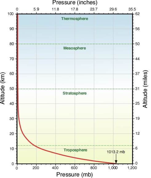
The Earth's atmosphere contains several different layers that can be defined according to air temperature, Figure 7b-1 displays these layers in an average atmosphere.

                    

Figure 7b-1: Vertical change in average global atmospheric temperature. Variations in the way temperature changes with height indicates the atmosphere is composed of a number of different layers (labeled above). These variations are due to changes in the chemical and physical characteristics of the atmosphere with altitude. 

According to temperature, the atmosphere contains four different layers (Figure 7b-1). The first layer is called the troposphere. The depth of this layer varies from about 8 to 16 kilometers. Greatest depths occur at the tropics where warm temperatures causes vertical expansion of the lower atmosphere. From the tropics to the Earth's polar regions the troposphere becomes gradually thinner. The depth of this layer at the poles is roughly half as thick when compared to the tropics. Average depth of the troposphere is approximately 11 kilometers as displayed in Figure 7b-1.

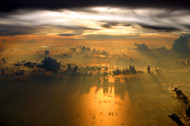
About 80% of the total mass of the atmosphere is contained in troposphere. It is also the layer where the majority of our weather occurs (Figure 7b-2). Maximum air temperature also occurs near the Earth's surface in this layer. With increasing height, air temperature drops uniformly with altitude at a rate of approximately 6.5° Celsius per 1000 meters. This phenomenon is commonly called the Environmental Lapse Rate. At an average temperature of -56.5° Celsius, the top of the troposphere is reached. At the upper edge of the troposphere is a narrow transition zone known as the tropopause.

Figure 7b-2: Most of our planet's weather occurs in the troposphere. This image shows a view of this layer from an airplane's window (Photo © 2004 Edward Tsang).

Above the tropopause is the stratosphere. This layer extends from an average altitude of 11 to 50 kilometers above the Earth's surface. This stratosphere contains about 19.9% of the total mass found in the atmosphere. Very little weather occurs in the stratosphere. Occasionally, the top portions of thunderstorms breach this layer. The lower portion of the stratosphere is also influenced by the polar jet stream and subtropical jet stream. In the first 9 kilometers of the stratosphere, temperature remains constant with height. A zone with constant temperature in the atmosphere is called an isothermal layer. 

From an altitude of 20 to 50 kilometers, temperature increases with an increase in altitude. The higher temperatures found in this region of the stratosphere occurs because of a localized concentration of ozone gas molecules. These molecules absorb ultraviolet sunlight creating heat energy that warms the stratosphere. Ozone is primarily found in the atmosphere at varying concentrations between the altitudes of 10 to 50 kilometers. This layer of ozone is also called the ozone layer . The ozone layer is important to organisms at the Earth's surface as it protects them from the harmful effects of the Sun's ultraviolet radiation. Without the ozone layer life could not exist on the Earth's surface.

Separating the mesosphere from the stratosphere is transition zone called the stratopause. In the mesosphere, the atmosphere reaches its coldest temperatures (about -90° Celsius) at a height of approximately 80 kilometers. At the top of the mesosphere is another transition zone known as the mesopause.

The last atmospheric layer has an altitude greater than 80 kilometers and is called the thermosphere. Temperatures in this layer can be greater than 1200° C. These high temperatures are generated from the absorption of intense solar radiation by oxygen molecules (O2). While these temperatures seem extreme, the amount of heat energy involved is very small. The amount of heat stored in a substance is controlled in part by its mass. The air in the thermosphere is extremely thin with individual gas molecules being separated from each other by large distances. 

Consequently, measuring the temperature of thermosphere with a thermometer is a very difficult process. Thermometers measure the temperature of bodies via the movement of heat energy. Normally, this process takes a few minutes for the conductive transfer of kinetic energy from countless molecules in the body of a substance to the expanding liquid inside the thermometer. In the thermosphere, our thermometer would lose more heat energy from radiative emission then what it would gain from making occasional contact with extremely hot gas molecules.

CITATION

Pidwirny, M. (2006). "The Layered Atmosphere". Fundamentals of Physical Geography, 2nd Edition. Date Viewed. http://www.physicalgeography.net/fundamentals/7b.html

ATMOSPHERIC COMPOSITION

Nitrogen and Oxygen are the main components of the atmosphere by volume. Together these two gases make up approximately 99% of the dry atmosphere. Both of these gases have very important associations with life. Nitrogen is removed from the atmosphere and deposited at the Earth's surface mainly by specialized nitrogen fixing bacteria, and by way of lightning through precipitation. The addition of this nitrogen to the Earth's surface soils and various water bodies supplies much needed nutrition for plant growth. Nitrogen returns to the atmosphere primarily through biomass combustion and denitrification.

Oxygen is exchanged between the atmosphere and life through the processes of photosynthesis and respiration. Photosynthesis produces oxygen when carbon dioxide and water are chemically converted into glucose with the help of sunlight. Respiration is a the opposite process of photosynthesis. In respiration, oxygen is combined with glucose to chemically release energy for metabolism. The products of this reaction are water and carbon dioxide.

The next most abundant gas on the table is water vapor. Water vapor varies in concentration in the atmosphere both spatially and temporally. The highest concentrations of water vapor are found near the equator over the oceans and tropical rain forests. Cold polar areas and subtropical continental deserts are locations where the volume of water vapor can approach zero percent. Water vapor has several very important functional roles on our planet:

• It redistributes heat energy on the Earth through latent heat energy exchange.
• The condensation of water vapor creates precipitation that falls to the Earth's surface providing needed fresh water for plants and animals.
• It helps warm the Earth's atmosphere through the greenhouse effect

The fifth most abundant gas in the atmosphere is carbon dioxide. The volume of this gas has increased by over 35% in the last three hundred years (see Figure 7a-1). This increase is primarily due to human induced burning from fossil fuels, deforestation, and other forms of land-use change. Carbon dioxide is an important greenhouse gas. The human-caused increase in its concentration in the atmosphere has strengthened the greenhouse effect and has definitely contributed to global warming over the last 100 years. Carbon dioxide is also naturally exchanged between the atmosphere and life through the processes of photosynthesis and respiration.

THE NATURAL SPHERE

From the standpoint of Physical Geography, the Earth can be seen to be composed of four principal components:

Lithosphere - describes the solid inorganic portion of the Earth (composed of rocks, minerals and elements). It can be regarded as the outer surface and interior of the solid Earth. On the surface of the Earth, the lithosphere is composed of three main types of rocks:

• Igneous - rocks formed by solidification of molten magma.
• Sedimentary - rocks formed by the alteration and compression of old rock debris or organic sediments.
• Metamorphic - rocks formed by alteration of existing rocks by intense heat or pressure.

Atmosphere - is the vast gaseous envelope of air that surrounds the Earth. Its boundaries are not easily defined. The atmosphere contains a complex system of gases and suspended particles that behave in many ways like fluids. Many of its constituents are derived from the Earth by way of chemical and biochemical reactions.

Hydrosphere - describes the waters of the Earth. Water exists on the Earth in various stores, including the atmosphere, oceans, lakes, rivers, soils, glaciers, and groundwater. Water moves from one store to another by way of evaporation, condensation, runoff, precipitation, infiltration and groundwater flow.

Biosphere - consists of all living things, plant and animal. This zone is characterized by life in profusion, diversity, and ingenious complexity. Cycling of matter in this sphere involves not only metabolic reactions in organisms, but also many abiotic chemical reactions.

All of these spheres are interrelated to each other by dynamic interactions, like biogeochemical cycling, that move and exchange both matter and energy between the four components.

CITATION

Pidwirny, M. (2006). "The Natural Spheres". Fundamentals of Physical Geography, 2nd Edition. 30/11/2011. http://www.physicalgeography.net/fundamentals/5c.html

THE UNIVERSE, EARTH, NATURAL SPHERE AND GAIA

(a) The Evolution of the Universe

About 11 to 15 billion years ago all of the matter and energy in the Universe was concentrated into an area the size of an atom. At this moment, matter, energy, space and time did not exist. Then suddenly, the Universe began to expand at an incredible rate and matter, energy, space and time came into being (the Big Bang). As the Universe expanded, matter began to coalesce into gas clouds, and then stars and planets. Our solar system formed about 5 billion years ago when the Universe was about 65% of its present size (Figure 5a-2). Today, the Universe continues to expand.

Figure 5a-2: Our solar system began forming about 5 billion years ago as gas clouds coalesce into planets and a star. Today, the solar system contains nine commonly recognized planets and the Sun. (Source: NASA).

THE SCIENCE OF PHYSICAL GEOGRAHPHY

(h) Inferential Statistics: Regression and Correlation Part C
1 There were 62 values of Y analyzed and therefore n = 62. The total sum of squares degrees of freedom (df) is determined as n-1 or 61. The regression of Y on X has 1 degree of freedom. The residual or unexplained degrees of freedom is determined by subtracting regression df (1) from total sum of squares df (61). 

2 MS is calculated as SS / df.

Using the Analysis of Variance procedure, the regression is tested by determining the calculated F statistic:

F = (Regression MS) / (Residual SS) = (2.1115) / (0.0112) = 188.86

To test this statistic we use a table of F to determine a critical test value for a probability of 0.01 or 1% (this relationship can occur by chance only in 1 out 100 cases) and with 1,60 degrees of freedom. According to the table the critical test value is 7.1. In this test, the relationship is deemed significant if the calculated F statistic is greater than the critical test value. This regression is statistically significant at the 0.01 level because 188.86 is greater than 7.1. 

Caution must be taken when interpreting the results of regression. In our example, we found a significant relationship between precipitation and cucumber yield. However, this conclusion may not be the result of a causal relationship between the two variables. A third variable that is directly associated to both precipitation and cucumber yield may be confounding the interpretation of the analysis. Absolute verification of associations between variables can only be confirmed with experimental manipulation.

Inferential Statistics: Regression and Correlation Part B

(h) Inferential Statistics: Regression and Correlation Part B

S X = 3,050

•  = 49.1935 

S Y = 26.62

•  = 0.4294 

n = 62

Often the first step in regression analysis is to plot the X and Y data on a graph (Figure 3h-1). This is done to graphically visualize the relationship between the two variables. If there is a simple relationship, the plotted points will have a tendancy to form a recognizable pattern (a straight line or curve). If the relationship is strong, the pattern will be very obvious. If the relationship is weak, the points will be more spread out and the pattern less distinct. If the points appear to fall pretty much at random, there may be no relationship between the two variables

 

 Figure 3h-1: Scattergram plot of the precipitation and cucumber yield data found in Table 3h-1. The distribution of the data points indicates a possible positive linear relationship between the two variables.

The type of pattern (straight line, parabolic curve, exponential curve, etc.) will determine the type of regression model to be applied to the data. In this particular case, we will examine data that produces a simple straight-line relationship (see Figure 3h-1). After selecting the model to be used, the next step is to calculate the corrected sums of squares and products used in a bivariate linear regression analysis. In the following equations, capital letters indicate uncorrected values of the variables and lower-case letters are used for the corrected parameters in the analysis.

The corrected sum of squares for Y:

S y2 = S Y2 -

= (0.362 + 0.092 + ... + 0.422) - (26.622) / 62

= 2.7826

The corrected sum of squares for X:

S x2 = S X2 -

= (222 + 62 + ... + 612) - (3,0502) / 62

= 59,397.6775

The corrected sum of products:

S xy = S (XY) -

= ((22)(.36) + (6)(.09) + ... + (61)(.42)) - ((26.62)(3,050)) / 62

= 354.1477

THE SCIENCE OF PHYSICAL GEOGRAPHY

(h) Inferential  Statistics: Regression and Correlation
Regression and correlation analysis are statistical techniques used extensively in physical geography to examine causal relationships between variables. Regression and correlation measure the degree of relationship between two or more variables in two different but related ways. In regression analysis, a single dependent variable, Y, is considered to be a function of one or more independent variables, X1, X2, and so on. 


The values of both the dependent and independent variables are assumed as being ascertained in an error-free random manner. Further, parametric forms of regression analysis assume that for any given value of the independent variable, values of the dependent variable are normally distributed about some mean. Application of this statistical procedure to dependent and independent variables produces an equation that "best" approximates the functional relationship between the data observations. 

Correlation analysis measures the degree of association between two or more variables. Parametric methods of correlation analysis assume that for any pair or set of values taken under a given set of conditions, variation in each of the variables is random and follows a normal distribution pattern. Utilization of correlation analysis on dependent and independent variables produces a statistic called the correlation coefficient (r). The square of this statistical parameter (the coefficient of determination or r2) describes what proportion of the variation in the dependent variable is associated with the regression of an independent variable. 

THE SCIENCE OF PHYSICAL GEOGRAPHY

(g) Inferential Statistics: Comparison of Sample Means
U = n1•n2 + {n1•(n1 + 1)}/2 - S r1 

U = 13 • 15 + {13•(13 + 1)}/2 - 267 = 19 

U1 = n1•n2 + {n2•(n2 + 1)}/2 - S r2
U1 = 13 • 15 + {15•(15 + 1)}/2 - 139 = 176

where n1 is the number of observations in the first sample, and n2 is the number of observations in the second sample.

The lower of these two values (U and U1) is then taken to determine the significance of the difference between the two data sets. Calculated from the data found on Table 3g-1, the value of U is 19 and U1 is 176. The lower value is thus 19. This value is now compared to the critical value found on the significance tables for the Mann-Whitney U (Table 3g-2) at a pre-determined significance level for the given sample sizes. An important feature of this statistical test is that the greater the difference between the two sets of samples, the smaller will be the test statistic (i.e., the lower value of U or U1). Thus, if the computed value is lower than the critical value in Table 3g-2, the null hypothesis (H0) is rejected for the given significance level. If the computed value is greater than the critical value, we then accept the null hypothesis.



Using a significance level of 0.05 with sample sizes of n1 = 13 and n2 = 15, the critical value in the table for a two-tailed test is 54. Note that this is a two-tailed test, because the direction of the relationship is not specified. The computed value of U is 19, which is much less than the tabulated value. Thus, the null hypothesis (H0) is rejected and the alternative hypothesis (H1) is accepted.

 Table 3g-2: Critical values of U for the Mann-Whitney U test (P = 0.05). 

n	1	2	3	4	5	6	7	8	9	10	11	12	13	14	15	16	17	18	19	20
1	-	-	-	-	-	-	-	-	-	-	-	-	-	-	-	-	-	-	-	-
2	-	-	-	-	-	-	-	0	0	0	0	1	1	1	1	1	2	2	2	2
3	-	-	-	-	0	1	1	2	2	3	3	4	4	5	5	6	6	7	7	8
4	-	-	-	-	-	-	3	4	4	5	6	7	8	9	10	11	11	12	13	13
5	-	0	1	2	2	3	5	6	7	8	9	10	12	13	14	15	17	18	19	20
6	-	-	-	-	-	5	6	8	10	11	13	14	16	17	19	21	22	24	25	27
7	-	-	-	-	-	-	8	10	12	14	16	18	20	22	24	26	28	30	32	34
8	-	-	-	-	-	-	-	13	15	17	19	22	24	26	29	31	34	36	38	41
9	-	-	-	-	-	-	-	-	17	20	23	26	28	31	34	37	39	42	45	48
10	-	-	-	-	-	-	-	-	-	23	26	29	33	36	39	42	45	48	52	55
11	-	-	-	-	-	-	-	-	-	-	30	33	37	40	44	47	51	55	58	62
12	-	-	-	-	-	-	-	-	-	-	-	37	41	45	49	53	57	61	65	69
13	-	-	-	-	-	-	-	-	-	-	-	-	45	50	54	59	63	67	72	76
14	-	-	-	-	-	-	-	-	-	-	-	-	-	55	59	64	67	74	78	83
15	-	-	-	-	-	-	-	-	-	-	-	-	-	-	64	70	75	80	85	90
16	-	-	-	-	-	-	-	-	-	-	-	-	-	-	-	75	81	86	92	98
17	-	-	-	-	-	-	-	-	-	-	-	-	-	-	-	-	87	93	99	105
18	-	-	-	-	-	-	-	-	-	-	-	-	-	-	-	-	-	99	106	112
19	-	-	-	-	-	-	-	-	-	-	-	-	-	-	-	-	-	-	113	119
20	-	-	-	-	-	-	-	-	-	-	-	-	-	-	-	-	-	-	-	127